1. What are decision trees and why would you use them?
decision trees are among the most popular classification algorithms;
they divide the dataset hierarchically starting from the full dataset, until the stop criterium is met, e.g. the minimum size of a leaf and the purity of leaf;
in general they are easy to understand, interpret and visualise
however they are not very efficient, but they can scale, i.e. they can be processed in parallel;
understanding decision trees is important if you want to learn random forests.
2. A few “hello world” examples
rpart
Calculating decision trees in R is rather straightforward. Probably the best known package which supports decision trees is rpart. Let’s have a look at a short example:
library(rpart)
tree <- rpart(Species ~ ., iris)

print(tree)
## n= 150
##
## node), split, n, loss, yval, (yprob)
## * denotes terminal node
##
## 1) root 150 100 setosa (0.33333333 0.33333333 0.33333333)
## 2) Petal.Length< 2.45 50 0 setosa (1.00000000 0.00000000 0.00000000) *
## 3) Petal.Length>=2.45 100 50 versicolor (0.00000000 0.50000000 0.50000000)
## 6) Petal.Width< 1.75 54 5 versicolor (0.00000000 0.90740741 0.09259259) *
## 7) Petal.Width>=1.75 46 1 virginica (0.00000000 0.02173913 0.97826087) *The summary above informs us, that the root (the whole dataset) was divided into two subsets, based on the value of the attribute Petal.Length. According to the docs (?print.rpart)
Information for each node includes the node number, split, size, deviance, and fitted value.
In our case, the root is classified as setosa, where among 150 observations 100 is classified incorrectly and there is 33% of setosa, versicolor and virginica each in this dataset.
Probably you will also be interested in the plot method:
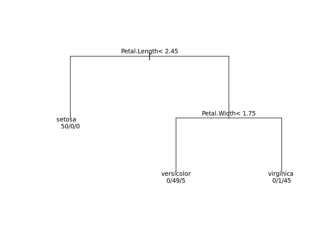
plot(tree, margin = 0.1)
text(tree, use.n = TRUE, cex = 0.75)
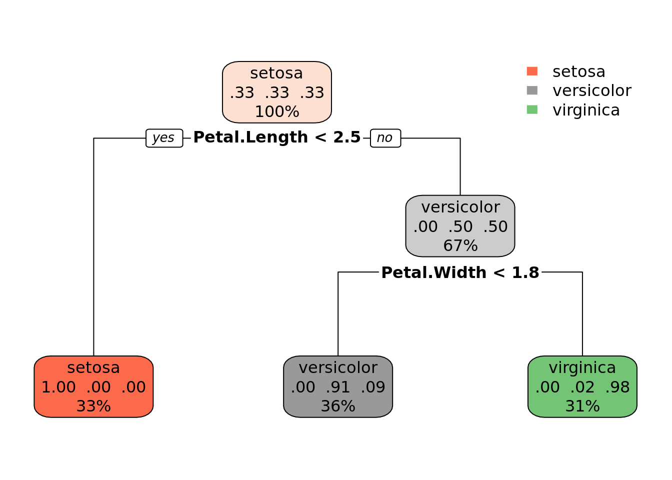
which produces a rather modest view of our tree. Luckily the are various packages, which can make the plot look more neat:
library(rpart.plot)
rpart.plot(tree)
decisionTree
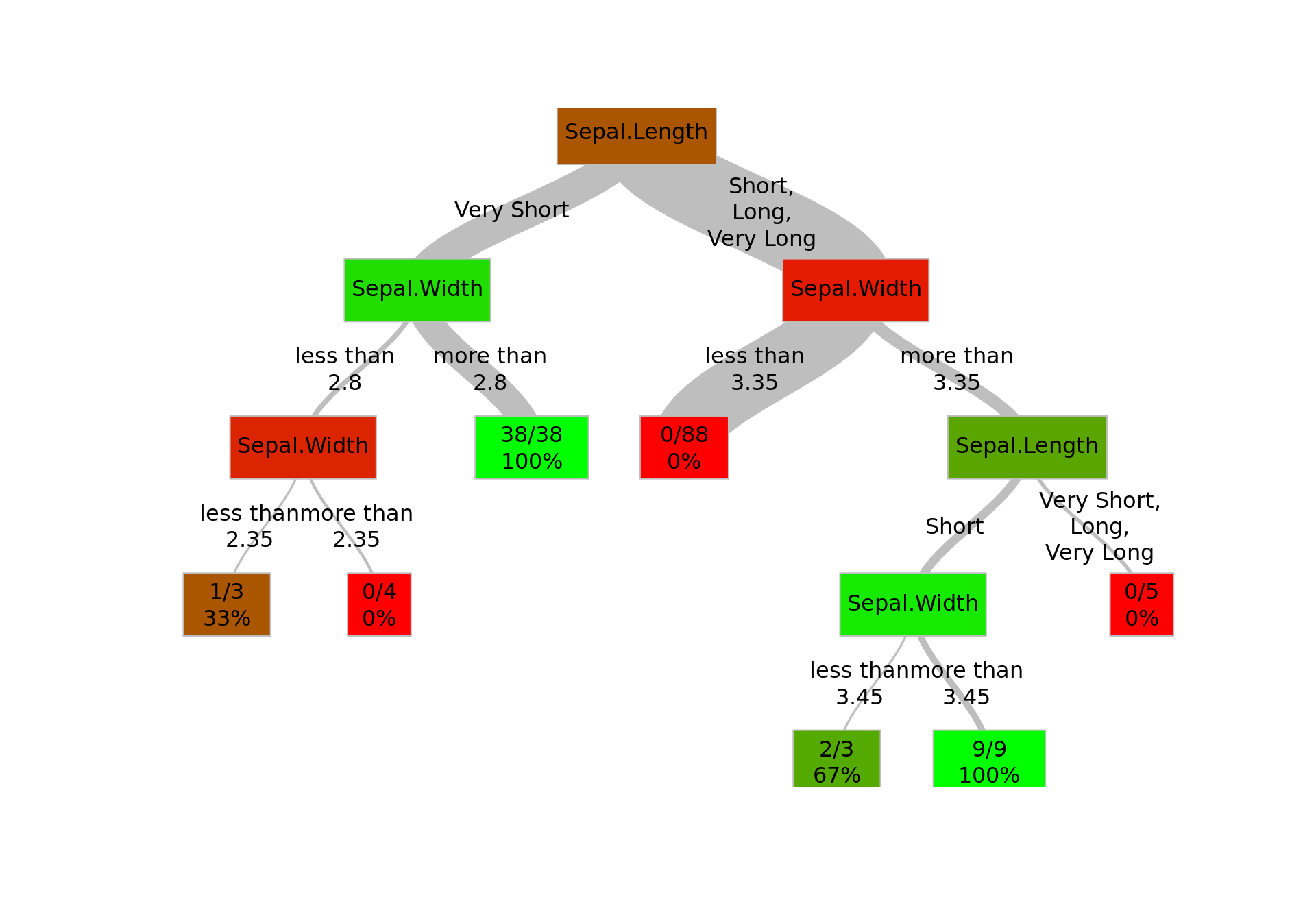
If you want to go really fancy, you can use my decisionTree package, which grows a decision tree for a binary response and has a legible plot method. The package is available at github, so you can download it easily with:
devtools::install_github('tomis9/decisionTree')First, let’s create a sample dataset based on iris dataset, which contains a binary response.
d <- iris[, c("Species", "Sepal.Length", "Sepal.Width")]
d$Species <- as.character(d$Species)
d$Species[d$Species != "setosa"] <- "non-setosa"
x <- d$Sepal.Length
x[d$Sepal.Length <= 5.2] <- "Very Short"
x[d$Sepal.Length >  5.2 & d$Sepal.Length <= 6.1] <- "Short"
x[d$Sepal.Length >  6.1 & d$Sepal.Length <= 7.0] <- "Long"
x[d$Sepal.Length >  7.0] <- "Very Long"
d$Sepal.Length <- x

summary(d)
## Species Sepal.Length Sepal.Width
## Length:150 Length:150 Min. :2.000
## Class :character Class :character 1st Qu.:2.800
## Mode :character Mode :character Median :3.000
## Mean :3.057
## 3rd Qu.:3.300
## Max. :4.400As you can see, the response variable is Species, which is binary. The other two values are independent; one of them is categorical, the other - continuous.
library(decisionTree)
tree <- decisionTree(d, eta = 5, purity=0.95, minsplit=0)
plot(tree)
