1. What is machine learning and why would you use it?
it’s a rather complicated, yet beautiful tool for boldly going where no man has gone before.
in other words, it enables you to extract valuable information from data.
2. Examples of the most popular machine learning algorithms in Python and R
We’ll be working on iris dataset, which is easily available in Python (from sklearn import datasets; datasets.load_iris()) and R (data(iris)).
We will use a few of the most popular machine learning tools:
R base,
R caret,
Python scikit-learn,
Python API to tensorflow.
tensorflowwas used in very few cases, because it is designed mainly for neural networks, and we would have to implement the algorithms from scratch.
Let’s prepare data for our algorithms. You can read more about data preparation in this blog post.
data preparation
Python
from sklearn import datasets
from sklearn.metrics import accuracy_score
from sklearn.model_selection import train_test_split

iris = datasets.load_iris()
X, y = iris.data, iris.target

X_train, X_test, y_train, y_test = train_test_split(
    X, y, test_size=0.33, random_state=42)

boston = datasets.load_boston()
# I will divide boston dataset to train and test later on
tensorflow
You can use functions from tensorflow_datasets module, but… does anybody use them?
base R
# unfortunately base R does not provide a function for train/test split
train_test_split <- function(test_size = 0.33, dataset) {
    smp_size <- floor(test_size * nrow(dataset))
    test_ind <- sample(seq_len(nrow(dataset)), size = smp_size)

    test <- dataset[test_ind, ]
    train <- dataset[-test_ind, ]
    return(list(train = train, test = test))
}

library(gsubfn)
## Warning: no DISPLAY variable so Tk is not availablelist[train, test] <- train_test_split(0.5, iris)caret R
# docs: ..., the random sampling is done within the
# levels of ‘y’ when ‘y’ is a factor in an attempt to balance the class
# distributions within the splits.
# I provide package's name before function's name for clarity
trainIndex <- caret::createDataPartition(iris$Species, p=0.7, list = FALSE,
times = 1)
train <- iris[trainIndex,]
test <- iris[-trainIndex,]SVM
The best description of SVM I found is in Data mining and analysis - Zaki, Meira. In general, I highly recommend this book.
Python
from sklearn.svm import SVC  # support vector classification

svc = SVC()
svc.fit(X_train, y_train)
## SVC(C=1.0, cache_size=200, class_weight=None, coef0=0.0,
## decision_function_shape='ovr', degree=3, gamma='auto_deprecated',
## kernel='rbf', max_iter=-1, probability=False, random_state=None,
## shrinking=True, tol=0.001, verbose=False)
##
## /usr/local/lib/python3.5/dist-packages/sklearn/svm/base.py:193: FutureWarning: The default value of gamma will change from 'auto' to 'scale' in version 0.22 to account better for unscaled features. Set gamma explicitly to 'auto' or 'scale' to avoid this warning.
## "avoid this warning.", FutureWarning)print(accuracy_score(svc.predict(X_test), y_test))## 1.0TODO: plotting svm in scikit
“base” R
svc <- e1071::svm(Species ~ ., train)

pred <- as.character(predict(svc, test[, 1:4]))
mean(pred == test["Species"])
## [1] 0.9555556caret R
svm_linear <- caret::train(Species ~ ., data = train, method = "svmLinear")
mean(predict(svm_linear, test) == test$Species)
## [1] 0.9777778decision trees
Python
from sklearn.tree import DecisionTreeClassifier

dtc = DecisionTreeClassifier()
dtc.fit(X_train, y_train)
## DecisionTreeClassifier(class_weight=None, criterion='gini', max_depth=None,
## max_features=None, max_leaf_nodes=None,
## min_impurity_decrease=0.0, min_impurity_split=None,
## min_samples_leaf=1, min_samples_split=2,
## min_weight_fraction_leaf=0.0, presort=False,
## random_state=None, splitter='best')print(accuracy_score(y_test, dtc.predict(X_test)))## 0.98TODO: an article on drawing decision trees in Python
“base” R
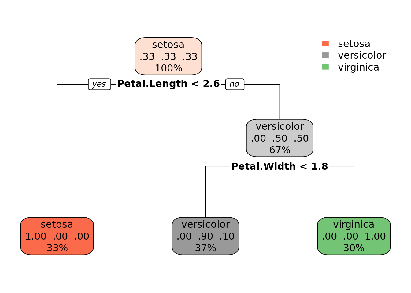
dtc <- rpart::rpart(Species ~ ., train)
print(dtc)
## n= 105
##
## node), split, n, loss, yval, (yprob)
## * denotes terminal node
##
## 1) root 105 70 setosa (0.3333333 0.3333333 0.3333333)
## 2) Petal.Length< 2.6 35 0 setosa (1.0000000 0.0000000 0.0000000) *
## 3) Petal.Length>=2.6 70 35 versicolor (0.0000000 0.5000000 0.5000000)
## 6) Petal.Width< 1.75 39 4 versicolor (0.0000000 0.8974359 0.1025641) *
## 7) Petal.Width>=1.75 31 0 virginica (0.0000000 0.0000000 1.0000000) *rpart.plot::rpart.plot(dtc)
pred <- predict(dtc, test[,1:4], type = "class")
mean(pred == test[["Species"]])
## [1] 0.9555556caret R
c_dtc <- caret::train(Species ~ ., train, method = "rpart")
print(c_dtc)
## CART
##
## 105 samples
## 4 predictor
## 3 classes: 'setosa', 'versicolor', 'virginica'
##
## No pre-processing
## Resampling: Bootstrapped (25 reps)
## Summary of sample sizes: 105, 105, 105, 105, 105, 105, ...
## Resampling results across tuning parameters:
##
## cp Accuracy Kappa
## 0.0000000 0.9500351 0.9241468
## 0.4428571 0.6705453 0.5221465
## 0.5000000 0.5329165 0.3248991
##
## Accuracy was used to select the optimal model using the largest value.
## The final value used for the model was cp = 0.rpart.plot::rpart.plot(c_dtc$finalModel)
I described working with decision trees in R in more detail in another blog post.
random forests
Python
from sklearn.ensemble import RandomForestClassifier

rfc = RandomForestClassifier()
rfc.fit(X_train, y_train)
## RandomForestClassifier(bootstrap=True, class_weight=None, criterion='gini',
## max_depth=None, max_features='auto', max_leaf_nodes=None,
## min_impurity_decrease=0.0, min_impurity_split=None,
## min_samples_leaf=1, min_samples_split=2,
## min_weight_fraction_leaf=0.0, n_estimators=10,
## n_jobs=None, oob_score=False, random_state=None,
## verbose=0, warm_start=False)
##
## /usr/local/lib/python3.5/dist-packages/sklearn/ensemble/forest.py:245: FutureWarning: The default value of n_estimators will change from 10 in version 0.20 to 100 in 0.22.
## "10 in version 0.20 to 100 in 0.22.", FutureWarning)print(accuracy_score(rfc.predict(X_test), y_test))## 0.98“base” R
rf <- randomForest::randomForest(Species ~ ., data = train)
mean(predict(rf, test[, 1:4]) == test[["Species"]])
## [1] 0.9555556caret R
c_rf <- caret::train(Species ~ ., train, method = "rf")
print(c_rf)
## Random Forest
##
## 105 samples
## 4 predictor
## 3 classes: 'setosa', 'versicolor', 'virginica'
##
## No pre-processing
## Resampling: Bootstrapped (25 reps)
## Summary of sample sizes: 105, 105, 105, 105, 105, 105, ...
## Resampling results across tuning parameters:
##
## mtry Accuracy Kappa
## 2 0.9581911 0.9364327
## 3 0.9580316 0.9362142
## 4 0.9599618 0.9391382
##
## Accuracy was used to select the optimal model using the largest value.
## The final value used for the model was mtry = 4.print(c_dtc$finalModel)## n= 105
##
## node), split, n, loss, yval, (yprob)
## * denotes terminal node
##
## 1) root 105 70 setosa (0.3333333 0.3333333 0.3333333)
## 2) Petal.Length< 2.6 35 0 setosa (1.0000000 0.0000000 0.0000000) *
## 3) Petal.Length>=2.6 70 35 versicolor (0.0000000 0.5000000 0.5000000)
## 6) Petal.Width< 1.75 39 4 versicolor (0.0000000 0.8974359 0.1025641) *
## 7) Petal.Width>=1.75 31 0 virginica (0.0000000 0.0000000 1.0000000) *knn
Python
from sklearn.neighbors import KNeighborsClassifier

knn = KNeighborsClassifier()
knn.fit(X, y)
## KNeighborsClassifier(algorithm='auto', leaf_size=30, metric='minkowski',
## metric_params=None, n_jobs=None, n_neighbors=5, p=2,
## weights='uniform')print(accuracy_score(y, knn.predict(X)))## 0.9666666666666667R
kn <- class::knn(train[,1:4], test[,1:4], cl = train[,5], k = 3)
mean(kn == test[,5])
## [1] 0.9555556TODO: caret r knn
kmeans
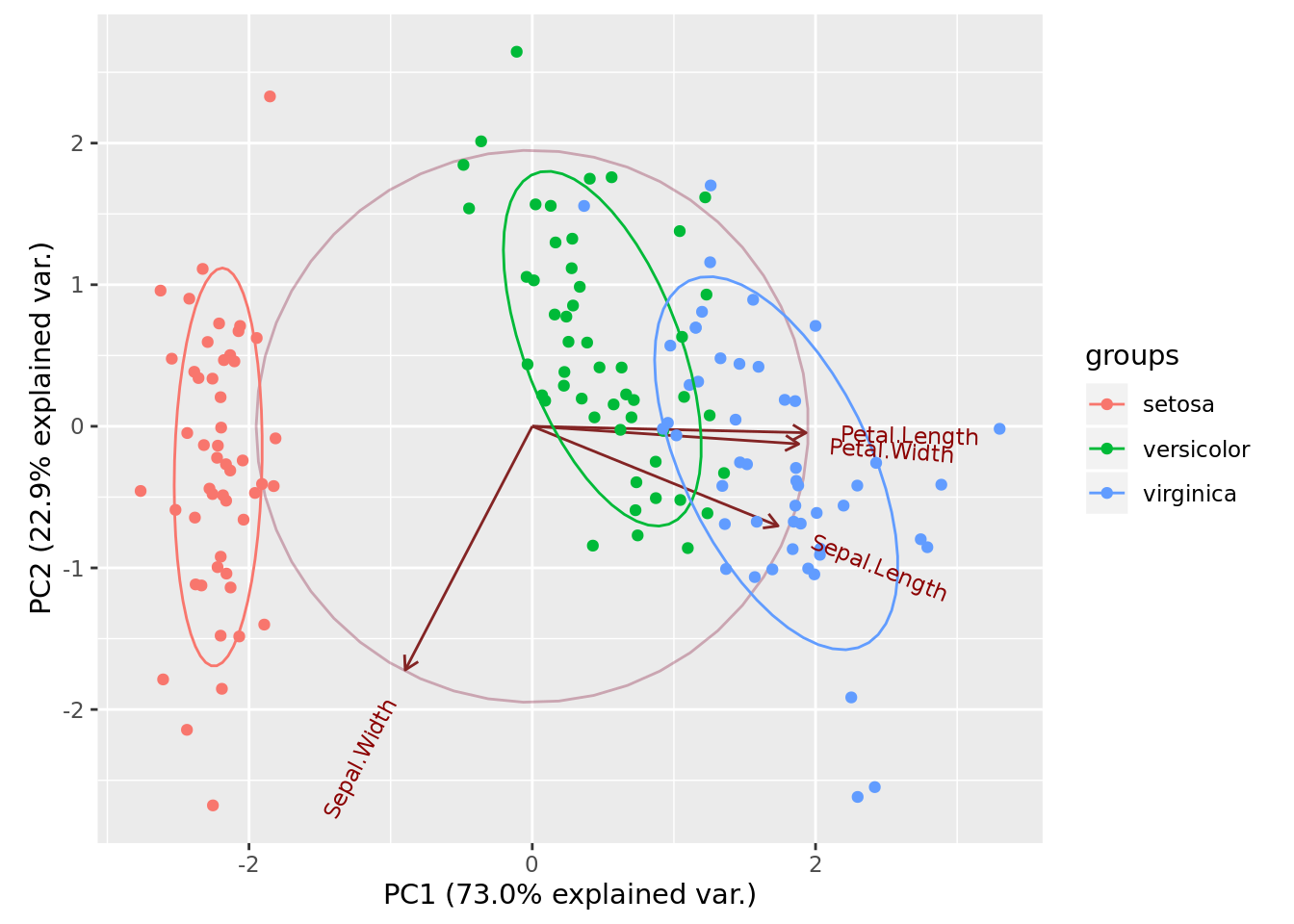
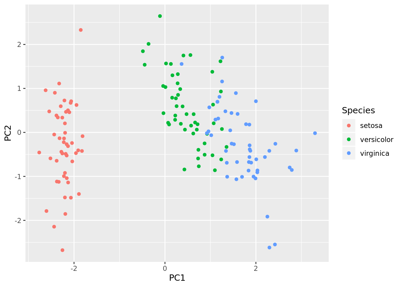
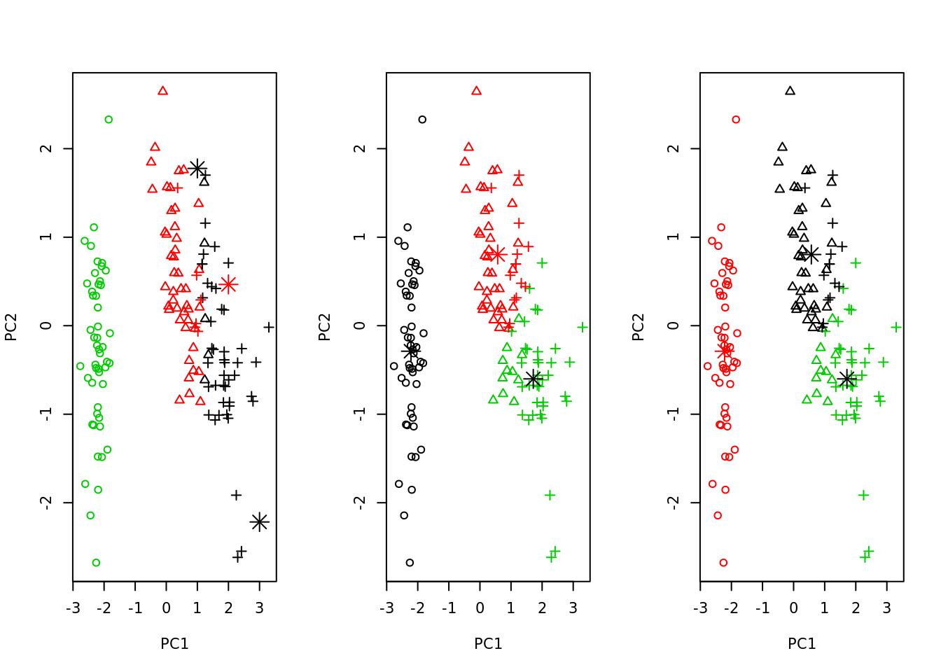
K-means can be nicely plotted in two dimensions with help of PCA.
R
pca <- prcomp(iris[,1:4], center = TRUE, scale. = TRUE)
# devtools::install_github("vqv/ggbiplot")
ggbiplot::ggbiplot(pca, obs.scale = 1, var.scale = 1, groups = iris$Species,
                   ellipse = TRUE, circle = TRUE)
iris_pca <- scale(iris[,1:4]) %*% pca$rotation
iris_pca <- as.data.frame(iris_pca)
iris_pca <- cbind(iris_pca, Species = iris$Species)

ggplot2::ggplot(iris_pca, aes(x = PC1, y = PC2, color = Species)) +
  geom_point()
plot_kmeans <- function(km, iris_pca) {
  # we choose only first two components, so they could be plotted
  plot(iris_pca[,1:2], col = km$cluster, pch = as.integer(iris_pca$Species))
  points(km$centers, col = 1:2, pch = 8, cex = 2)
}
par(mfrow=c(1, 3))
# we use 3 centers, because we already know that there are 3 species
sapply(list(kmeans(iris_pca[,1], centers = 3),
            kmeans(iris_pca[,1:2], centers = 3),
            kmeans(iris_pca[,1:4], centers = 3)),
       plot_kmeans, iris_pca = iris_pca)
## [[1]]
## NULL
##
## [[2]]
## NULL
##
## [[3]]
## NULL
interesting article - kmeans with dplyr and broom
TODO: caret r - kmeans
TODO: python - kmeans
linear regression
Python
from sklearn.linear_model import LinearRegression
from sklearn import datasets

X, y = boston.data, boston.target

lr = LinearRegression()
lr.fit(X, y)
## LinearRegression(copy_X=True, fit_intercept=True, n_jobs=None, normalize=False)print(lr.intercept_)## 36.45948838509017print(lr.coef_)
# TODO calculate this with iris dataset## [-1.08011358e-01 4.64204584e-02 2.05586264e-02 2.68673382e+00
## -1.77666112e+01 3.80986521e+00 6.92224640e-04 -1.47556685e+00
## 3.06049479e-01 -1.23345939e-02 -9.52747232e-01 9.31168327e-03
## -5.24758378e-01]tensorflow
- data preparation
import tensorflow as tf## /usr/local/lib/python3.5/dist-packages/tensorflow/python/framework/dtypes.py:516: FutureWarning: Passing (type, 1) or '1type' as a synonym of type is deprecated; in a future version of numpy, it will be understood as (type, (1,)) / '(1,)type'.
## _np_qint8 = np.dtype([("qint8", np.int8, 1)])
## /usr/local/lib/python3.5/dist-packages/tensorflow/python/framework/dtypes.py:517: FutureWarning: Passing (type, 1) or '1type' as a synonym of type is deprecated; in a future version of numpy, it will be understood as (type, (1,)) / '(1,)type'.
## _np_quint8 = np.dtype([("quint8", np.uint8, 1)])
## /usr/local/lib/python3.5/dist-packages/tensorflow/python/framework/dtypes.py:518: FutureWarning: Passing (type, 1) or '1type' as a synonym of type is deprecated; in a future version of numpy, it will be understood as (type, (1,)) / '(1,)type'.
## _np_qint16 = np.dtype([("qint16", np.int16, 1)])
## /usr/local/lib/python3.5/dist-packages/tensorflow/python/framework/dtypes.py:519: FutureWarning: Passing (type, 1) or '1type' as a synonym of type is deprecated; in a future version of numpy, it will be understood as (type, (1,)) / '(1,)type'.
## _np_quint16 = np.dtype([("quint16", np.uint16, 1)])
## /usr/local/lib/python3.5/dist-packages/tensorflow/python/framework/dtypes.py:520: FutureWarning: Passing (type, 1) or '1type' as a synonym of type is deprecated; in a future version of numpy, it will be understood as (type, (1,)) / '(1,)type'.
## _np_qint32 = np.dtype([("qint32", np.int32, 1)])
## /usr/local/lib/python3.5/dist-packages/tensorflow/python/framework/dtypes.py:525: FutureWarning: Passing (type, 1) or '1type' as a synonym of type is deprecated; in a future version of numpy, it will be understood as (type, (1,)) / '(1,)type'.
## np_resource = np.dtype([("resource", np.ubyte, 1)])
## /usr/local/lib/python3.5/dist-packages/tensorboard/compat/tensorflow_stub/dtypes.py:541: FutureWarning: Passing (type, 1) or '1type' as a synonym of type is deprecated; in a future version of numpy, it will be understood as (type, (1,)) / '(1,)type'.
## _np_qint8 = np.dtype([("qint8", np.int8, 1)])
## /usr/local/lib/python3.5/dist-packages/tensorboard/compat/tensorflow_stub/dtypes.py:542: FutureWarning: Passing (type, 1) or '1type' as a synonym of type is deprecated; in a future version of numpy, it will be understood as (type, (1,)) / '(1,)type'.
## _np_quint8 = np.dtype([("quint8", np.uint8, 1)])
## /usr/local/lib/python3.5/dist-packages/tensorboard/compat/tensorflow_stub/dtypes.py:543: FutureWarning: Passing (type, 1) or '1type' as a synonym of type is deprecated; in a future version of numpy, it will be understood as (type, (1,)) / '(1,)type'.
## _np_qint16 = np.dtype([("qint16", np.int16, 1)])
## /usr/local/lib/python3.5/dist-packages/tensorboard/compat/tensorflow_stub/dtypes.py:544: FutureWarning: Passing (type, 1) or '1type' as a synonym of type is deprecated; in a future version of numpy, it will be understood as (type, (1,)) / '(1,)type'.
## _np_quint16 = np.dtype([("quint16", np.uint16, 1)])
## /usr/local/lib/python3.5/dist-packages/tensorboard/compat/tensorflow_stub/dtypes.py:545: FutureWarning: Passing (type, 1) or '1type' as a synonym of type is deprecated; in a future version of numpy, it will be understood as (type, (1,)) / '(1,)type'.
## _np_qint32 = np.dtype([("qint32", np.int32, 1)])
## /usr/local/lib/python3.5/dist-packages/tensorboard/compat/tensorflow_stub/dtypes.py:550: FutureWarning: Passing (type, 1) or '1type' as a synonym of type is deprecated; in a future version of numpy, it will be understood as (type, (1,)) / '(1,)type'.
## np_resource = np.dtype([("resource", np.ubyte, 1)])from sklearn.datasets import load_iris
import numpy as np
def get_data(tensorflow=True):
iris = load_iris()
data = iris.data
y = data[:, 0].reshape(150, 1)
x0 = np.ones(150).reshape(150, 1)
X = np.concatenate((x0, data[:, 1:]), axis=1)
if tensorflow:
y = tf.constant(y, name='y')
X = tf.constant(X, name='X') # constant is a tensor
return X, y- using normal equations
def construct_beta_graph(X, y):
    cov = tf.matmul(tf.transpose(X), X, name='cov')
    inv_cov = tf.matrix_inverse(cov, name='inv_cov')
    xy = tf.matmul(tf.transpose(X), y, name='xy')
    beta = tf.matmul(inv_cov, xy, name='beta')
    return beta


X, y = get_data()
beta = construct_beta_graph(X, y)
mse = tf.reduce_mean(tf.square(y - tf.matmul(X, beta)))

init = tf.global_variables_initializer()
with tf.Session() as sess:
    init.run()
    print(beta.eval())
    print(mse.eval())
## [[ 1.85599749]
## [ 0.65083716]
## [ 0.70913196]
## [-0.55648266]]
## 0.09630269942460729- using gradient descent and mini-batches
learning_rate = 0.01
n_iter = 1000

X_train, y_train = get_data(tensorflow=False)

X = tf.placeholder("float64", shape=(None, 4))  # placeholder -
y = tf.placeholder("float64", shape=(None, 1))

start_values = tf.random_uniform([4, 1], -1, 1, dtype="float64")
beta = tf.Variable(start_values, name='beta')
mse = tf.reduce_mean(tf.square(y - tf.matmul(X, beta)))

optimizer = tf.train.GradientDescentOptimizer(learning_rate=learning_rate)
_training = optimizer.minimize(mse)

batch_indexes = np.arange(150).reshape(5,30)

init = tf.global_variables_initializer()
with tf.Session() as sess:
    init.run()
    for i in range(n_iter):
        for batch_index in batch_indexes:
            _training.run(feed_dict={X: X_train[batch_index],
                                     y: y_train[batch_index]})
        if not i % 100:
            print(mse.eval(feed_dict={X: X_train, y: y_train}))
    print(mse.eval(feed_dict={X: X_train, y: y_train}), "- final score")
    print(beta.eval())
## 2.3895152369649946
## 0.10797717245831852
## 0.10373690497710132
## 0.10151411027702137
## 0.1002318517147055
## 0.09941500533633553
## 0.0988476858681415
## 0.09842729043262417
## 0.09810184472808979
## 0.09784279281501808
## 0.0976348605920062 - final score
## [[ 1.51170067]
## [ 0.7385839 ]
## [ 0.73761717]
## [-0.58416114]]base R
model <- lm(Sepal.Length ~ ., train)
summary(model)
##
## Call:
## lm(formula = Sepal.Length ~ ., data = train)
##
## Residuals:
## Min 1Q Median 3Q Max
## -0.64990 -0.19821 0.02046 0.21233 0.67506
##
## Coefficients:
## Estimate Std. Error t value Pr(>|t|)
## (Intercept) 1.95948 0.31803 6.161 1.56e-08 ***
## Sepal.Width 0.54600 0.09536 5.726 1.11e-07 ***
## Petal.Length 0.82000 0.08097 10.127 < 2e-16 ***
## Petal.Width -0.01272 0.17011 -0.075 0.940539
## Speciesversicolor -0.94541 0.26745 -3.535 0.000622 ***
## Speciesvirginica -1.52013 0.36870 -4.123 7.79e-05 ***
## ---
## Signif. codes: 0 '***' 0.001 '**' 0.01 '*' 0.05 '.' 0.1 ' ' 1
##
## Residual standard error: 0.297 on 99 degrees of freedom
## Multiple R-squared: 0.871, Adjusted R-squared: 0.8645
## F-statistic: 133.7 on 5 and 99 DF, p-value: < 2.2e-16lm() function automatically converts factor variables to one-hot encoded features.
R caret
library(caret)

m <- train(Sepal.Length ~ ., data = train, method = "lm")
summary(m)  # exactly the same as lm()
##
## Call:
## lm(formula = .outcome ~ ., data = dat)
##
## Residuals:
## Min 1Q Median 3Q Max
## -0.64990 -0.19821 0.02046 0.21233 0.67506
##
## Coefficients:
## Estimate Std. Error t value Pr(>|t|)
## (Intercept) 1.95948 0.31803 6.161 1.56e-08 ***
## Sepal.Width 0.54600 0.09536 5.726 1.11e-07 ***
## Petal.Length 0.82000 0.08097 10.127 < 2e-16 ***
## Petal.Width -0.01272 0.17011 -0.075 0.940539
## Speciesversicolor -0.94541 0.26745 -3.535 0.000622 ***
## Speciesvirginica -1.52013 0.36870 -4.123 7.79e-05 ***
## ---
## Signif. codes: 0 '***' 0.001 '**' 0.01 '*' 0.05 '.' 0.1 ' ' 1
##
## Residual standard error: 0.297 on 99 degrees of freedom
## Multiple R-squared: 0.871, Adjusted R-squared: 0.8645
## F-statistic: 133.7 on 5 and 99 DF, p-value: < 2.2e-16logistic regression
In these examples I will present classification of a dummy variable.
Python
from sklearn.linear_model import LogisticRegression

cond = iris.target != 2
X = iris.data[cond]
y = iris.target[cond]

X_train, X_test, y_train, y_test = train_test_split(
    X, y, test_size=0.33, random_state=42)

lr = LogisticRegression()

lr.fit(X_train, y_train)
## LogisticRegression(C=1.0, class_weight=None, dual=False, fit_intercept=True,
## intercept_scaling=1, l1_ratio=None, max_iter=100,
## multi_class='warn', n_jobs=None, penalty='l2',
## random_state=None, solver='warn', tol=0.0001, verbose=0,
## warm_start=False)
##
## /usr/local/lib/python3.5/dist-packages/sklearn/linear_model/logistic.py:432: FutureWarning: Default solver will be changed to 'lbfgs' in 0.22. Specify a solver to silence this warning.
## FutureWarning)accuracy_score(lr.predict(X_test), y_test)## 1.0base R
species <- c("setosa", "versicolor")
d <- iris[iris$Species %in% species,]
d$Species <- factor(d$Species, levels = species)
library(gsubfn)
list[train, test] <- train_test_split(0.5, d)

m <- glm(Species ~ Sepal.Length, train, family = binomial)
# predictions - if prediction is bigger than 0.5, we assume it's a one,
# or success
y_hat_test <- predict(m, test[,1:4], type = "response") > 0.5

# glm's doc:
# For ‘binomial’ and ‘quasibinomial’ families the response can also
# be specified as a ‘factor’ (when the first level denotes failure
# and all others success) or as a two-column matrix with the columns
# giving the numbers of successes and failures.
# in our case - species[1] ("setosa") is a failure (0) and species[2]
# ("versicolor") is 1 (success)
# successes:
y_test <- test$Species == species[2]

mean(y_test == y_hat_test)
## [1] 0.9R caret
library(caret)
m2 <- train(Species ~ Sepal.Length, data = train, method = "glm", family = binomial)
mean(predict(m2, test) == test$Species)
## [1] 0.9xgboost
Python
from xgboost import XGBClassifier

cond = iris.target != 2
X = iris.data[cond]
y = iris.target[cond]

X_train, X_test, y_train, y_test = train_test_split(
    X, y, test_size=0.33, random_state=42)

xgb = XGBClassifier()
xgb.fit(X_train, y_train)
## XGBClassifier(base_score=0.5, booster='gbtree', colsample_bylevel=1,
## colsample_bynode=1, colsample_bytree=1, gamma=0,
## learning_rate=0.1, max_delta_step=0, max_depth=3,
## min_child_weight=1, missing=None, n_estimators=100, n_jobs=1,
## nthread=None, objective='binary:logistic', random_state=0,
## reg_alpha=0, reg_lambda=1, scale_pos_weight=1, seed=None,
## silent=None, subsample=1, verbosity=1)accuracy_score(xgb.predict(X_test), y_test)## 1.0“base” R
species <- c("setosa", "versicolor")
d <- iris[iris$Species %in% species,]
d$Species <- factor(d$Species, levels = species)
library(gsubfn)
list[train, test] <- train_test_split(0.5, d)

library(xgboost)
m <- xgboost(
  data = as.matrix(train[,1:4]),
  label = as.integer(train$Species) - 1,
  objective = "binary:logistic",
  nrounds = 2)
## [1] train-error:0.000000
## [2] train-error:0.000000mean(predict(m, as.matrix(test[,1:4])) > 0.5) == (as.integer(test$Species) - 1)## [1] FALSE FALSE FALSE FALSE FALSE FALSE FALSE FALSE FALSE FALSE FALSE
## [12] FALSE FALSE FALSE FALSE FALSE FALSE FALSE FALSE FALSE FALSE FALSE
## [23] FALSE FALSE FALSE FALSE FALSE FALSE FALSE FALSE FALSE FALSE FALSE
## [34] FALSE FALSE FALSE FALSE FALSE FALSE FALSE FALSE FALSE FALSE FALSE
## [45] FALSE FALSE FALSE FALSE FALSE FALSETODO: R: xgb.save(), xgb.importance()
caret R
