1. What is nls and why would you use it?

• nls, or nonlinear least squares is a statistical method used to describe a process as a nonlinear function of deterministic variables and a random variable;

• you may think of it as an older and stronger brother of linear regression - more robust, powerful, smarter and difficult to understand ;)

2. A “Hello World” example

Let’s assume we want to model US population as a function of year.

USPop <- data.frame(
  year = seq(from = 1790, to = 2000, by = 10),
  population = c(3.929, 5.308, 7.240, 9.638, 12.861, 17.063, 23.192, 31.443, 
                 38.558, 50.189, 62.980, 76.212, 92.228, 106.022, 123.203, 
                 132.165, 151.326, 179.323, 203.302, 226.542, 248.710, 281.422)
)

plot(population ~ year, data = USPop, 
     main = "US population over the last 200 years or so")
abline(lm(population ~ year, data = USPop), col = "red", lwd = 2)

USPop dataset used to be available in car package, curiously it isn’t anymore.

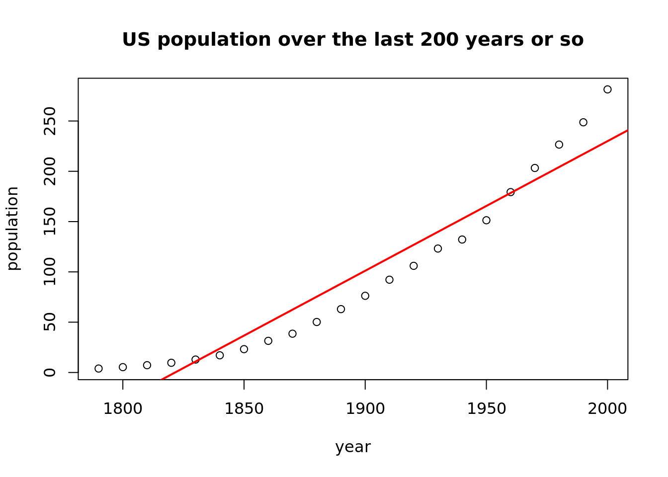
Yeah, I love these statistical, ascetic plots. The black line is a line proposed by linear regression and as we can see, it does not really fit the data. We can observe a rising trend, but it definitely is not linear. Modeling this process as a nonlinear function of year seems to be a reasonable approach.

But what kind of nonlinear function should we use? One of the most popular nonlinear functions is a logistic function. In this case we will use it’s more general form, in which the maximum value of the function is not 1, but \(\theta_1\):

\[ f(\textrm{year}) = \frac{\theta_1}{1 + e^{-(\theta_2 + \theta_3 * \textrm{year})}} \]

Before we’ll move to the estimation of the parameters, let’s calculate starting values for minimisation (least squares) algorithm. A natural candidate would be coefficients of a linear regression, where our dependant variable is linearised with a logit() function. Note that is the linearised model we will not extimate the Intercept, as we scale the dependant variable by diving all the values by a little more than it’s maximum, so that \(\textrm{population}\in(0,1)\). Our estimation of the Intercept is this maximum value that we divided by.

t1 <- max(USPop$population) * 1.05
model_start <- lm(car::logit(population / t1) ~ year, USPop)
starts <- c(t1, model_start$coefficients)
names(starts) <- c("theta1", "theta2", "theta3")
print(starts)

##       theta1       theta2       theta3 
## 295.49310000 -57.46319522   0.02968818

Let’s estimate the model coefficients using nls() function.

form <- population ~ theta1  / (1 + exp(-(theta2 + theta3 * year)))
model <- nls(formula = form, data = USPop, start = starts)
print(model)

## Nonlinear regression model
##   model: population ~ theta1/(1 + exp(-(theta2 + theta3 * year)))
##    data: USPop
##    theta1    theta2    theta3 
## 440.83109 -42.70710   0.02161 
##  residual sum-of-squares: 457.8
## 
## Number of iterations to convergence: 7 
## Achieved convergence tolerance: 7.273e-06

As we can observe, the estimated parameters’ values do not differ much from starting values.

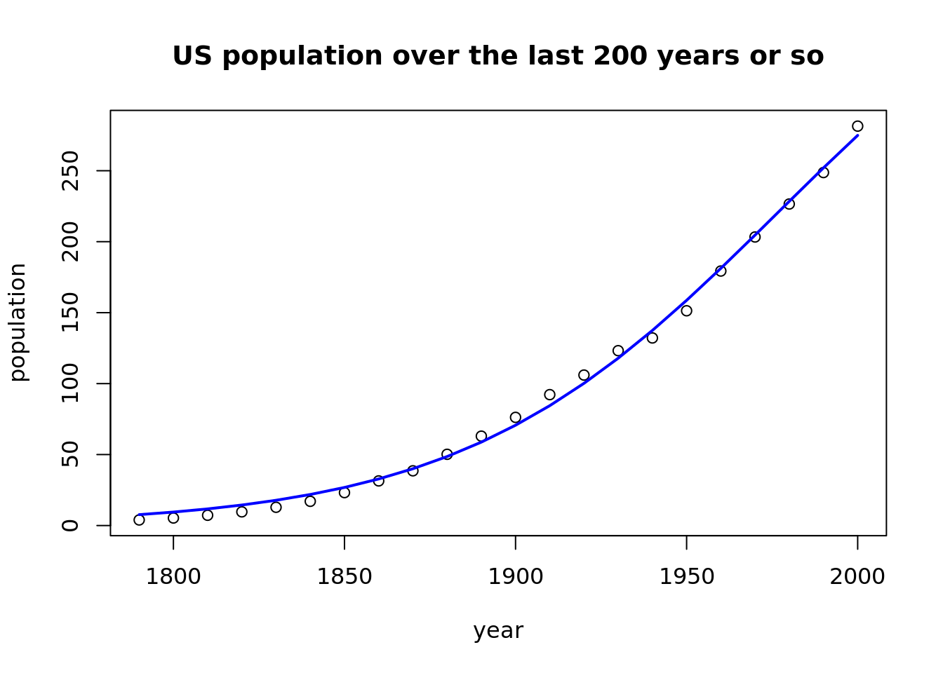
The plot below presents a much better fit of a model with logistic function, comparing to linear regression.

plot(population ~ year, data = USPop, 
     main = "US population over the last 200 years or so")
USPop$fitted_values <- fitted(model)
lines(fitted_values ~ year, data = USPop, col = "blue", lwd = 2)

3. Afterthoughts

• using nls() in fact does not differ much from using standard ls();

• we can use any function, not only logistic regerssion.