1. What is model validation and why would you do it?
You learned your model and naturally you are wondering how good it is. There are several ways to find out, like measuring the accuracy of predictions, but you may also want to check where exactly particular predictions come from, as this is far from obvious for “black box” models.
2. Examples
cross-validation
confusion matrix
https://www.rdocumentation.org/packages/caret/versions/3.45/topics/confusionMatrix
Confusion matrix is confusing at all as the name may suggest.
base R
dataset preparation (described in more detail here)
# prepare the dataset
library(caret)
## Loading required package: lattice## Loading required package: ggplot2species <- c("setosa", "versicolor")
d <- iris[iris$Species %in% species,]
d$Species <- factor(d$Species, levels = species)
trainIndex <- caret::createDataPartition(d$Species, p=0.7, list = FALSE,
times = 1)
train <- d[trainIndex,]
test <- d[-trainIndex,]
y_test <- test$Species == species[2]and the logistic regression itself:
m <- glm(Species ~ Sepal.Length, train, family = "binomial")
y_hat_test <- predict(m, test[,1:4], type = "response") > 0.5
We’ve prepared our predictions, as well as testing target, as vectors of binary values:
y_test[1:10]## [1] FALSE FALSE FALSE FALSE FALSE FALSE FALSE FALSE FALSE FALSEy_hat_test[1:10]## 1 9 13 16 19 24 26 28 38 40
## FALSE FALSE FALSE TRUE TRUE FALSE FALSE FALSE FALSE FALSEso now we may use a simple table() function to create a confusion matrix:
table(y_hat_test, y_test)## y_test
## y_hat_test FALSE TRUE
## FALSE 13 2
## TRUE 2 13- R caret
caret provides a much broader summary of confusion matrix:
library(caret)
m2 <- train(Species ~ Sepal.Length, train, method = "glm", family = binomial)
confusionMatrix(predict(m2, test), test$Species)
## Confusion Matrix and Statistics
##
## Reference
## Prediction setosa versicolor
## setosa 13 2
## versicolor 2 13
##
## Accuracy : 0.8667
## 95% CI : (0.6928, 0.9624)
## No Information Rate : 0.5
## P-Value [Acc > NIR] : 2.974e-05
##
## Kappa : 0.7333
##
## Mcnemar's Test P-Value : 1
##
## Sensitivity : 0.8667
## Specificity : 0.8667
## Pos Pred Value : 0.8667
## Neg Pred Value : 0.8667
## Prevalence : 0.5000
## Detection Rate : 0.4333
## Detection Prevalence : 0.5000
## Balanced Accuracy : 0.8667
##
## 'Positive' Class : setosa
## from sklearn.datasets import load_iris
from sklearn.model_selection import train_test_split
from sklearn.linear_model import LogisticRegression
from sklearn.metrics import accuracy_score, confusion_matrix
iris = load_iris()
cond = iris.target != 0
X = iris.data[cond]
y = iris.target[cond]
X_train, X_test, y_train, y_test = train_test_split(
X, y, test_size=0.33, random_state=42)
lr = LogisticRegression()
lr.fit(X_train, y_train)## LogisticRegression(C=1.0, class_weight=None, dual=False, fit_intercept=True,
## intercept_scaling=1, l1_ratio=None, max_iter=100,
## multi_class='warn', n_jobs=None, penalty='l2',
## random_state=None, solver='warn', tol=0.0001, verbose=0,
## warm_start=False)
##
## /usr/local/lib/python3.5/dist-packages/sklearn/linear_model/logistic.py:432: FutureWarning: Default solver will be changed to 'lbfgs' in 0.22. Specify a solver to silence this warning.
## FutureWarning)accuracy_score(lr.predict(X_test), y_test)## 0.9090909090909091print(confusion_matrix(lr.predict(X_test), y_test))## [[16 0]
## [ 3 14]]ROC, AUC
Let’s say you created a simple classifier, e.g. using logistic regression. The classifier does not return classes though, but the probability that this particular observation belongs to class 1. As what we need are classes, not probabilities, we have to somehow map these probabilities into classes. The easiest way to achieve this is by using a function like:
\[ f(t) = \begin{cases} 1 & \text{when $p \geqslant t$} \\ 0 & \text{when $p < t$} \\ \end{cases} \]
where \(t\) is a threshold set by you. Choose wisely ;)
Choosing a proper value of \(t\) is known as a “Precision / Recall tradeoff”:
A wonderful article about AUC and ROC curves. There is no nedd to duplicate it.
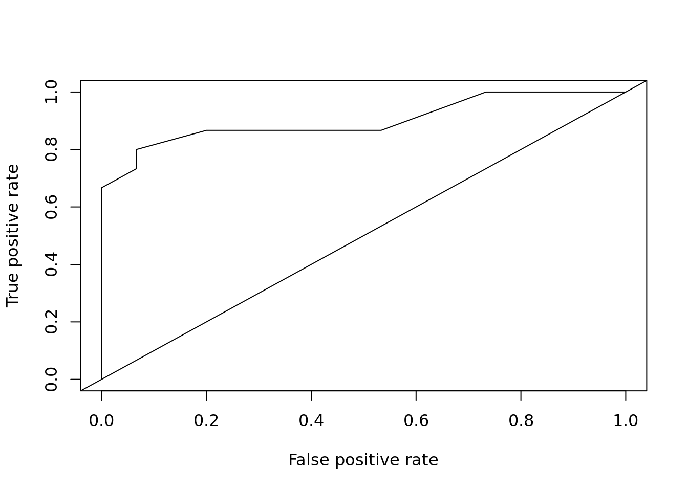
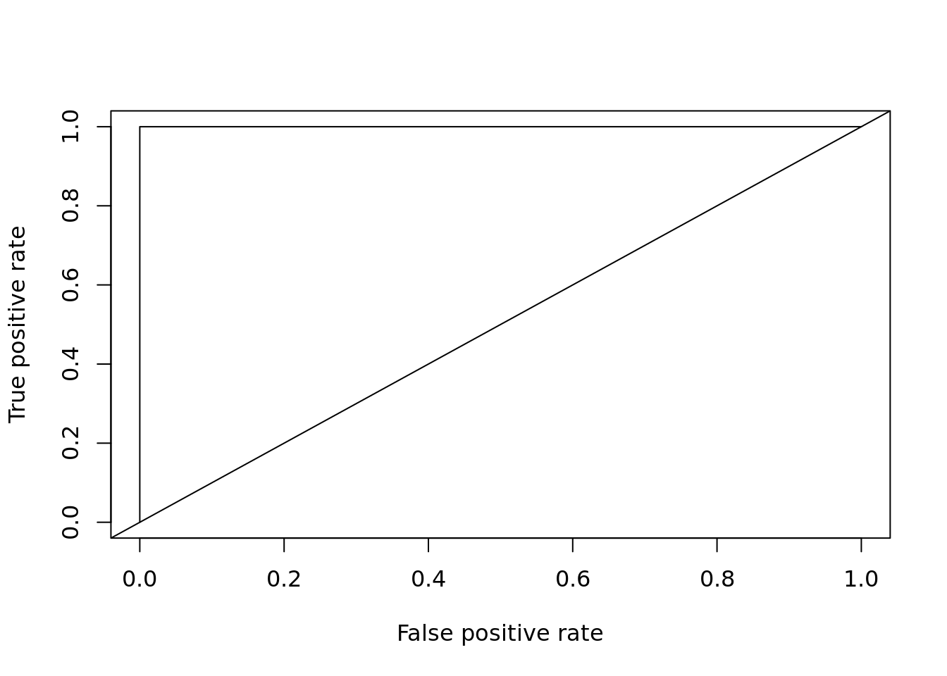
Different values of TPR and FPR for various \(t\) create a ROC curve. Area Under this Curve is called AUC.
R - using ROCR package
library(ROCR)
plot_roc_get_auc <- function(pred, test_labels) {
  roc_pred <- ROCR::prediction(pred, test_labels)
  roc_perf <- ROCR::performance(roc_pred, measure = "tpr", x.measure = "fpr")
  ROCR::plot(roc_perf, col = 1:10)
  abline(a = 0, b = 1)
  auc_perf <- ROCR::performance(roc_pred, measure = "auc", x.measure = "fpr")
  return(auc_perf@y.values[[1]])
}

species <- c("setosa", "versicolor")
iris_bin <- iris[iris$Species %in% species,]
iris_bin$Species <- factor(iris_bin$Species, levels = species)
trainIndex <- caret::createDataPartition(iris_bin$Species, p=0.7, list = FALSE,
                                         times = 1)
train <- iris_bin[trainIndex,]
test <- iris_bin[-trainIndex,]


m <- glm(Species ~ Sepal.Length, train, family = binomial)
plot_roc_get_auc(
  pred = predict(m, test[,1:4], type = "response"),
  test_labels = as.integer(test[["Species"]]) - 1)
## [1] 0.9rf <- randomForest::randomForest(Species ~ ., data = train)
plot_roc_get_auc(
pred = predict(rf, test[, 1:4], type = "prob")[,'versicolor'],
test_labels = as.integer(test[["Species"]]) - 1)
## [1] 1ROC - TPR vs FPR, where
\[ \textrm{TPR} = \frac{\textrm{TP}}{\textrm{TP} + \textrm{FP}} \]
TPR - True Positive Rate TP - True Positive FP - False Positive
parameter search
https://scikit-learn.org/stable/modules/grid_search.html#tuning-the-hyper-parameters-of-an-estimator
TODO: https://rviews.rstudio.com/2019/03/01/some-r-packages-for-roc-curves/
TODO: https://www.saedsayad.com/model_evaluation_c.htm
